Notes on Simple and Multiple Logistic Regression
If you have binary response (e.g., Natural vs. Technological) logistic regression can be a good choice for modeling. But remember two things: For resppnses with more than two categories, you can use multinomial logistic regression but it does not give you reliable estimates and its too many assumptions might be difficult to check. Moreover, make sure the response is actually binanry not continious as dichotomizing continious variables is a problematic practice.
Now We want to predcit Natural and Technological categories of stimuli using Valence and Arousal.
threats <- read.csv("https://raw.githubusercontent.com/soheilshapouri/affect_disasters/main/Data%20S2.csv")
threats <- threats[,c("Valence_Scaled", "Arousal_Scaled", "DisasterGroup")]
colnames(threats) <- c("Valence", "Arousal", "DisasterGroup")
threats$DisasterGroup <- as.factor(threats$DisasterGroup)
Before moving forward, I would check the response as unequal categories of response can be an issue.
table(threats$DisasterGroup)
imbalance classes of outcomes tells me I should use strtified sampling instead of simple random sampling to assute that they have same proportions in train-test splits as original data. (alternatively I can sample in a way that natural and technological stimuli have same proprtions).
threats_split <- initial_split(threats, prop = .8, strata = DisasterGroup)
threats_train <- training(threats_split)
threats_test <- testing(threats_split)
Start with a simple logistic regression
model1 <- glm(DisasterGroup ~ Valence, family = "binomial", data = threats_train)
confint(model1)
levels(threats_train$DisasterGroup)
exp(coef(model1))
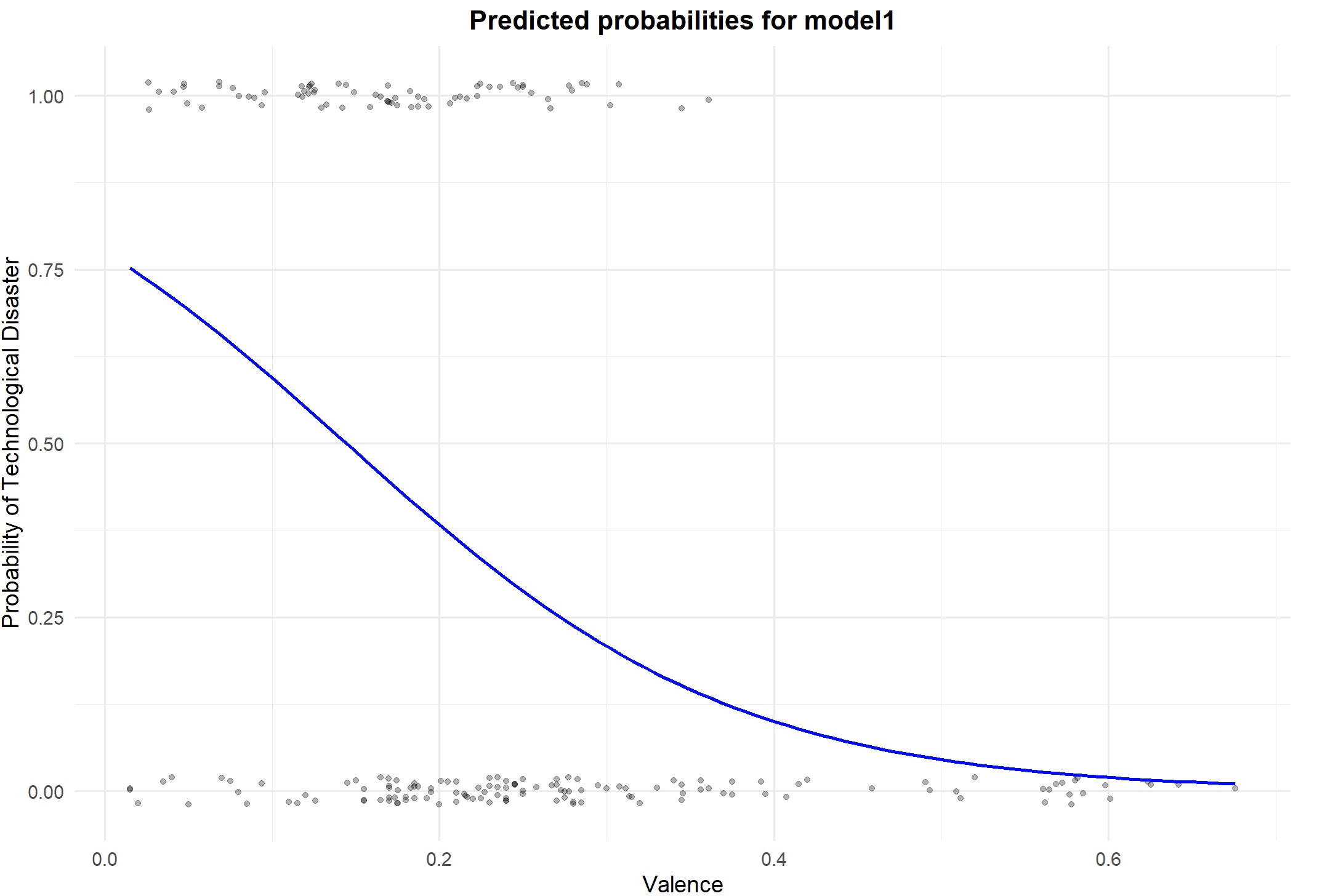
The significant coefficient and natural being the reference category (so technological as modeling category) say there is a negative relationship betwen valence and being technological. As stimuli become more pleasant it is less lekiely to belong to technological category. changing the logit scale, For a 1-unit increase in Valence, the odds of being in the “Technological” group (relative to “Natural”) decrease by a factor of 0.0002. The relationship can be shown by the graph below.
# Load necessary libraries
library(ggplot2)

# Create a sequence of Valence values for prediction
valence_seq <- seq(min(threats_train$Valence), max(threats_train$Valence), length.out = 100)

# Create a data frame for predictions
prediction_data <- data.frame(Valence = valence_seq)

# Predict probabilities using model1
prediction_data$Probability <- predict(model1, newdata = prediction_data, type = "response")

# Plot the predicted probabilities
ggplot(data = threats_train, aes(x = Valence, y = as.numeric(DisasterGroup == "Technological"))) +
  geom_jitter(height = 0.02, alpha = 0.3) +  # Add jittered points for data visualization
  geom_line(data = prediction_data, aes(x = Valence, y = Probability), color = "blue", size = 1) +  # Prediction line
  labs(
    title = "Predicted probabilities for model1",
    x = "Valence",
    y = "Probability of Technological Disaster"
  ) +
  theme_minimal(base_size = 14) +
  theme(
    plot.title = element_text(face = "bold", size = 16, hjust = 0.5),
    axis.title = element_text(size = 14)
  )
 We can also fit a simple logistic regression with arousal instead of valence
model2 <- glm(DisasterGroup ~ Arousal, family = "binomial", data = threats_train)
summary(model2)
Basically, same pattern here. As arousal increases th eporbability of a stimilus being technological decreases.
Now, move to multiple logistic regression.
model3 <- glm(DisasterGroup ~ Valence + Arousal, family = "binomial", data = threats_train)
summary(model3)
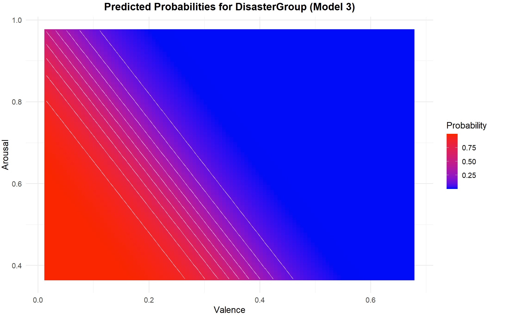
The codes and graph for visualization of multiple logistic regression are below but the graph would be more interesting if we had a continious and a categorical predictor.
library(ggplot2)
library(dplyr)

# Create a grid of Valence and Arousal values for predictions
valence_seq <- seq(min(threats_train$Valence), max(threats_train$Valence), length.out = 100)
arousal_seq <- seq(min(threats_train$Arousal), max(threats_train$Arousal), length.out = 100)

# Create a data frame with all combinations of Valence and Arousal
grid <- expand.grid(Valence = valence_seq, Arousal = arousal_seq)

# Predict probabilities using model3
grid$Probability <- predict(model3, newdata = grid, type = "response")

# Plot the predicted probabilities as a contour plot
ggplot(grid, aes(x = Valence, y = Arousal, z = Probability)) +
  geom_tile(aes(fill = Probability)) +
  geom_contour(color = "white", alpha = 0.7) +
  scale_fill_gradient(low = "blue", high = "red", name = "Probability") +
  labs(
    title = "Predicted Probabilities for DisasterGroup (Model 3)",
    x = "Valence",
    y = "Arousal"
  ) +
  theme_minimal(base_size = 14) +
  theme(
    plot.title = element_text(face = "bold", size = 16, hjust = 0.5),
    axis.title = element_text(size = 14)
  )
 Now that we know the basics of logistic regression, we do it much more sophisticated with cross-validation to better evaluate them.
model1_cv <- train(
  form = DisasterGroup ~ Valence,
  data = threats_train,
  method = "glm",
  family = "binomial",
  trControl = trainControl(method = "cv", number = 10)
)


model2_cv <- train(
  form = DisasterGroup ~ Arousal,
  data = threats_train,
  method = "glm",
  family = "binomial",
  trControl = trainControl(method = "cv", number = 10)
  )


model3_cv <- train(
  form = DisasterGroup ~ .,
  data = threats_train,
  method = "glm",
  family = "binomial",
  trControl = trainControl(method = "cv", number = 10)
)

summary(
  resamples(
    list(model1_cv, model2_cv, model3_cv)
  )
)
Obviously, model 3 with the mean accuracy of .81 is better than others. But we can also use ROC plots to compare models.
library(ROCR)
library(dplyr)
# Compute predicted probabilities
m1_prob <- predict(model1_cv, threats_train, type = "prob")$Technological
m3_prob <- predict(model3_cv, threats_train, type = "prob")$Technological

# Compute AUC metrics for model1_cv and model3_cv
perf1 <- prediction(m1_prob, threats_train$DisasterGroup) %>%
  performance(measure = "tpr", x.measure = "fpr")
perf2 <- prediction(m3_prob, threats_train$DisasterGroup) %>%
  performance(measure = "tpr", x.measure = "fpr")

# Plot ROC curves for cv_model1 and cv_model3
plot(perf1, col = "black", lty = 2)
plot(perf2, add = TRUE, col = "blue")
legend(0.8, 0.2, legend = c("cv_model1", "cv_model3"),
       col = c("black", "blue"), lty = 2:1, cex = 0.6)
By comparing AUC in ROC plots we see, once again, than model 3 is better. So, we further evaluate that one. Considering the imbalance of natural and technological classes, if I always predict natural, I will be correct most of the time. So, I will show that model 3 is much better when we use it to predict the minority category.
pred_class <- predict(model3_cv, threats_train)

confusionMatrix(
  data = relevel(pred_class, ref = "Technological"),
  reference = relevel(threats_train$DisasterGroup, ref = "Technological")
)
The code above shows No Information Rate of 0.6471 which is basically the proportion of natural in the train set. Simply by predicting natural we would be right in 65 percent of cases. Model 3 was better than that as it does a good job regarding minority class. By AUC in ROC plots, comparing accuracy of models, and showing that it was better than merely predicting majority class the model seems good. Meanwhile the sensitivity of the model is relatively low at 0.6944, meaning the model correctly identifies only about 69% of the Technological cases. While the specificity (accuracy for identifying Natural cases) is higher at 0.8939, the lower sensitivity indicates room for improvement in detecting Technological events. Possible solutions:
- Weighted Logistic Regression: Assign higher weights to “Technological” cases during model training to penalize misclassification.
- Regularization (Penalized Logistic Regression)
- add interaction term (Valence:Arousal) to logistic regression
Finally, one thing I would check is multicolinearity as I know typically valence and arousal are correlted.library(car) vif(model3_cv$finalModel)becuase of multicolinearity I would also check PLS method to reduce dimentions.
set.seed(123)
cv_model_pls <- train(
DisasterGroup ~ .,
data = threats_train,
method = "pls",
family = "binomial",
trControl = trainControl(method = "cv", number = 10),
tuneLength = 2
)
In this case, its accuracy was not much higher. Before wraping up, remember to use finalModel instead of model3 for final evaluations with testing set.