Decision Trees
Decision trees might not be the first choice wehn it comes to predictive accuracy, but they have some advantages over other methods that make them a good choice you should always consider:
- They do not require transformation prior to modeling
- They are resistant to outliers
- They can handle missing values
So, let’s grow some trees to predcit collectivism from ecological factors.
ecodata <- read.csv("https://raw.githubusercontent.com/soheilshapouri/epidemics_collectivism/main/Data%20S2.csv")
library(rsample)
set.seed(123)
ecodata_split <- initial_split(ecodata, prop = 0.8, strata = "GCI")
ecodata_train <- training(ecodata_split)
ecodata_test <- testing(ecodata_split)
Decision trees with rpart package
eco_dt1 <- rpart(
  formula = GCI ~ No_Epidemics + No_Disasters + Death_Epidemics + Death_Disasters + Mortality_Epidemics + Mortality_Disasters + GDP + Region,
  data = ecodata_train,
  method = "anova"
)
# method = "anova" for regression problems, method = "class" for classification problems
If you are only concerned about predictive accuracy, multicolinearity is not an issue here. So, I entered all the predicotrs I had in the data.
eco_dt1
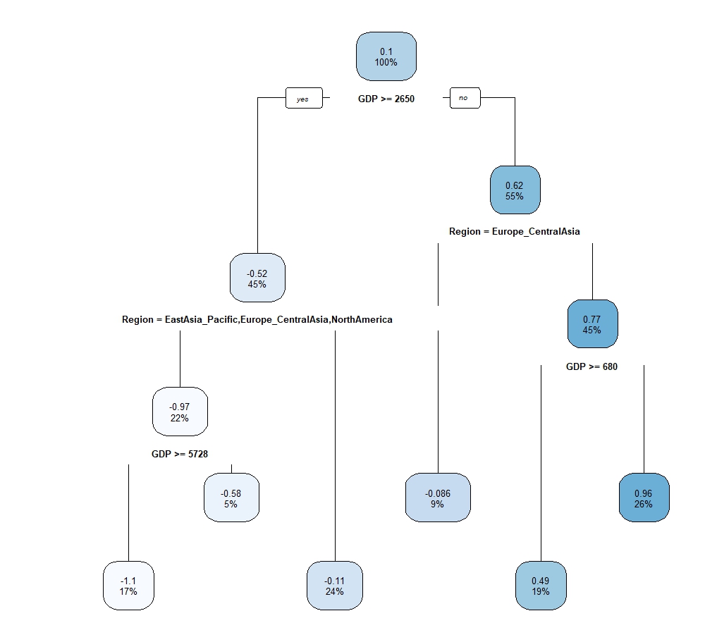
The output shows GDP is the first variable resulting in the largest reduction of SSE. But it is more intuitive to look at the visualization of decision trees.
Visualization
library(rpart.plot)
rpart.plot(eco_dt1)

As always better to train decision trees with caret package to do cross-validation. The hyperparameter that should be considered above is Complexity Parameter (cp). Tune Length = 20 means 20 different values will be considered for cp.
eco_dt2 <- train(
  GCI ~ No_Epidemics + No_Disasters + Death_Epidemics + Death_Disasters + Mortality_Epidemics + Mortality_Disasters + GDP + Region,
  data = ecodata_train,
  method = "rpart",
  trControl = trainControl(method = "cv", number = 10, savePredictions = "all"),
  tuneLength = 20
)
You get the warning message that “There were missing values in resampled performance measures” as in some categories of Region like North America there are not enough data fro providing evaluation metrics.
Model Evaluation
summary(eco_dt2$resample)
The output of the summary shows average perfromace (R2, RMSE) across 10 folds. What I see is that it was not better than ordinary least squares. Two more decision trees with different predictors to make some important conclusions.
eco_dt3 <- train(
  GCI ~ No_Epidemics + No_Disasters + GDP + Region,
  data = ecodata_train,
  method = "rpart",
  trControl = trainControl(method = "cv", number = 10, savePredictions = "all"),
  tuneLength = 20
)
summary(eco_dt3$resample)

eco_dt4 <- train(
  GCI ~ No_Epidemics + No_Disasters + GDP,
  data = ecodata_train,
  method = "rpart",
  trControl = trainControl(method = "cv", number = 10, savePredictions = "all"),
  tuneLength = 20
)
summary(eco_dt4$resample)

eco_dt5 <- train(
  GCI ~ GDP + Region,
  data = ecodata_train,
  method = "rpart",
  trControl = trainControl(method = "cv", number = 10, savePredictions = "all"),
  tuneLength = 20
)
summary(eco_dt5$resample)
Removing many predictors like number of epidecmis, deaths, and mortality didn’t lower the performance, but removing region does, and it does that significantly. That’s the importance of including the random effect which I will address in another post.